Bayesian Networks – BayesFusion

What are Bayesian Networks?

Bayesian networks (BNs) (also called belief networks, belief nets, or causal networks), introduced by Judea Pearl (1988), is a graphical formalism for representing joint probability distributions. Based on the fundamental work on the representation of and reasoning with probabilistic independence, originated by a British statistician A. Philip Dawid in 1970s, Bayesian networks offer an intuitive and efficient way of representing sizable domains, making modeling of complex systems practical. Bayesian networks provide a convenient and coherent way to represent uncertainty in uncertain models and are increasingly used for representing uncertain knowledge. It is not an overstatement to say that the introduction of Bayesian networks has changed the way we think about probabilities.

If you want to see Bayesian network models in action, visit our interactive model repository at https://repo.bayesfusion.com. The repository is accessible in any modern web browser and does not require any additional software installation.

We also recommend short articles on two extensions of Bayesian networks: dynamic Bayesian networks and influence diagrams.

The theoretical minimum

Bayesian networks are acyclic directed graphs that represent factorizations of joint probability distributions. Every joint probability distribution over n random variables can be factorized in n! ways and written as a product of probability distributions of each of the variables conditional on other variables. Consider a simple model consisting of four variables Socio-Economic Status (E), Smoking (S), Asbestos Exposure (A), and Lung Cancer (C). The joint probability distribution over these four variables can be factorized in 4!=24 ways, for example,

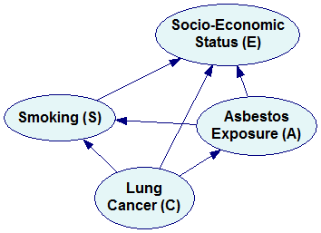
Each of these factorizations can be represented by a Bayesian network. We construct the directed graph of the network by creating a node for each of the factors in the distribution (we label each of the nodes with the name of a variable before the conditioning bar) and drawing directed arcs between them, always from the variables on the right hand side of the conditioning bar to the variable on the left hand side. For the first factorization above

Pr(E,S,A,C)=Pr(E|S,A,C) Pr(S|A,C) Pr(A|C) Pr(C)

we will construct the following Bayesian network:

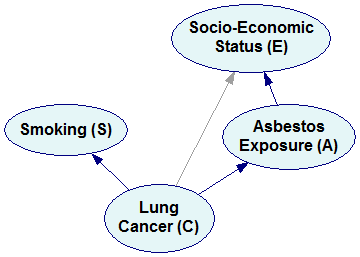
The fourth factorization

Pr(E,S,A,C)=Pr(C|E,S,A) Pr(A|E,S) Pr(S|E) Pr(E)

will yield the following Bayesian network:

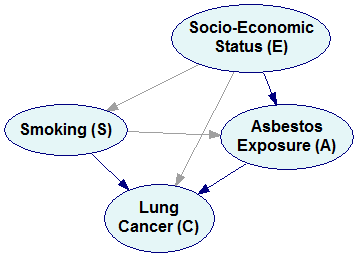
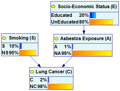
Please note that we have an arc from E to S because there is a factor Pr(S|E) in the factorization. Arcs from S, E, and A to C correspond to the factor Pr(C|E,S,A).

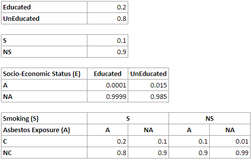
A graph tells us much about the structure of a probabilistic domain but not much about its numerical properties. These are encoded in conditional probability distribution matrices (equivalent to the factors in the factorized form), called conditional probability tables (CPTs) that are associated with the nodes. It is worth noting that there will always be nodes in the network with no predecessors. These nodes are characterized by their prior marginal probability distribution. Any probability in the joint probability distribution can be determined from these explicitly represented prior and conditional probabilities.

For the network above, we will have the following CPTs for the nodes E, S, A and C respectively:

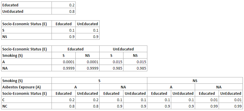
A straightforward representation of the join probability distribution over n binary variables requires us to represent the probability of every combination of states of these variables. For n binary variables, for example, we have 2^n-1 such combinations. In the example network above, we need 2^4-1=15 numerical parameters. While there are 30 numbers in the four tables above, please note that half of them are implied by other parameters, as the sum of all probabilities in every distribution has to be 1.0, which makes the total number of independent parameters 15.

Now, suppose that we know that Socio-Economic Status and Smoking are independent of each other. If so, then knowing whether somebody is educated or not tells us nothing about this person’s smoking status. Formally, we have Pr(S|E)=Pr(S). This allows us to simplify the factorization to the following

Pr(E,S,A,C)=Pr(C|E,S,A) Pr(A|E,S) Pr(S) Pr(E)

Similarly, suppose that we know that Asbestos Exposure and Smoking are independent of each other. If so, then knowing whether somebody smokes or not tells us nothing about this person’s exposure to asbestos. Formally, we have Pr(A|S)=Pr(A). This allows us to further simplify the factorization to the following

Pr(E,S,A,C)=Pr(C|E,S,A) Pr(A|E) Pr(S) Pr(E)

Finally, supposed that we realize that knowledge of Smoking status and Asbestos Exposure makes Socio-Economic Status irrelevant to the probability of Cancer, i.e., Pr(C|E,S,A)= Pr(C|S,A). We can simplify the factorization further to

Pr(E,S,A,C)=Pr(C|S,A) Pr(A|E) Pr(S) Pr(E)

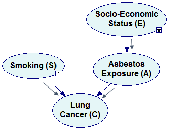
The Bayesian network representing the simplified factorization looks as follows:

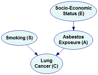
Please note that the new network is missing three arcs compared to the original network (marked by dimmed arcs in the previous pictures). These three arcs correspond to three independences that we encoded in the simplified factorization. It is a general rule that every independence between a pair of variables results in a missing arc. Conversely, if two nodes are not directly connected by an arc, then there exists such set of variables in the joint probability distribution that makes them conditionally independent. A possible interpretation of this is that the variables are not directly dependent. If we need to condition on other variables to make them independent, then they are indirectly dependent.

Let us look at the conditional probability tables encoded in the simplified network:

This simpler network contains fewer numerical parameters, as the CPTs for the nodes Smoking, Lung Cancer and Asbestos Exposure are smaller. The total number of parameters is 16 and the total number of independent parameters is only 8. This reduction in the number of parameters necessary to represent a joint probability distribution through an explicit representation of independences is the key feature of Bayesian networks.

Of all the factorizations possible, those that are capable of representing all independences known in the domain are preferable. Please note that the three independences that we were aware of, Pr(S|E)=Pr(S), Pr(A|S)=Pr(A) and Pr(C|E,S,A)= Pr(C|S,A) could not be captured by each of the possible factorizations. For example, in case of the first factorization

Pr(E,S,A,C)=Pr(E|S,A,C) Pr(S|A,C) Pr(A|C) Pr(C)

there is no way we could capture the independence Pr(C|E,S,A)= Pr(C|S,A) and the factorization can be simplified to only

Pr(E,S,A,C)=Pr(E|A,C) Pr(S|C) Pr(A|C) Pr(C)

which corresponds to the following Bayesian network:

Using independences to simplify the graphical model is a general principle that leads to simple, efficient representations of joint probability distributions. As an example, consider the following Bayesian network, modeling various problems encountered in diagnosing Diesel locomotives, their possible causes, symptoms, and test results.

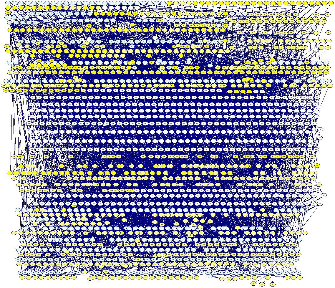
This network contains 2,127 nodes, i.e., it models a joint probability distribution over 2,127 variables. Given that each of the variables is binary, to represent this distribution in a brute force way, we would need 2^2127, which is around 10^632 numbers. To make the reader aware of the magnitude of this number, we would like to point out that the currently held estimate for the number of atoms in the universe is merely 10^82, which is 550 orders of magnitude smaller than 10^632, i.e., it would require a many parameters as the number of atoms in 10^550 universes like ours. The model pictured above is represented by only 6,433 independent parameters. As we can see, representing joint probability distributions becomes practical and models of the size of the example above are not uncommon.

A less formal (although also perfectly sound) view

The purely theoretical view that Bayesian networks represent independences and that lack of an arc between any two variables X and Y represents a (possibly conditional) independence between them, is not intuitive and convenient in practice. A popular, slightly informal view of Bayesian networks is that they represent causal graphs in which every arc represents a direct causal influence between the variables that it connects. A directed arc from X to Y captures the knowledge that X is a causal factor for Y. While this view is informal and it is easy to construct mathematically correct counter-examples, it is convenient and widely used by almost everybody applying Bayesian networks in practice. There is a well-established assumption, with no convincing counter-examples, that causal graphs will automatically lead to correct patterns of independences. Please recall the Bayesian network constructed in the previous section. Its arcs correspond to the intuitive notions that Smoking and Asbestos Exposure can cause Lung Cancer and that Socio-Economic Status influences Asbestos Exposure. Lack of arcs between pairs of variables expresses simple facts about absence of causal influences between them. Independences between these pairs of variables follow from the structure of the graph. It is, thus, possible to construct Bayesian networks based purely on our understanding of causal relations between variables in our model.

Reasoning with Bayesian networks

Structural properties of Bayesian networks, along with the conditional probability tables associated with their nodes allow for probabilistic reasoning within the model. Probabilistic reasoning within a BN is induced by observing evidence. A node that has been observed is called an evidence node. Observed nodes become instantiated, which means, in the simplest case, that their outcome is known with certainty. The impact of the evidence can be propagated through the network, modifying the probability distribution of other nodes that are probabilistically related to the evidence. For the example network, modeling various causes of Lung Cancer, we can answer questions like What is the probability of lung cancer in an educated smoker?, What is the probability of asbestos exposure in a lung cancer patient?, or Which question should we ask next?

In case of the first question, we instantiate the variables Smoking and Socio-Economic Status to S and Educated respectively and perform update of the network. The evidence entered can be visualized as spreading across the network.

This process amounts at the foundations to a repetitive application of Bayes theorem in order to update the probability distributions of all nodes in the network. Different ways of applying Bayes theorem and different order of updating lead to different algorithms. Essentially, the existing algorithms for reasoning in Bayesian networks can be divided into three groups: message passing, graph reduction, and stochastic simulation. Explicit representation of independences allows for an increased computational tractability of probabilistic reasoning. Probabilistic inference in singly connected BNs is very efficient. Unfortunately, exact algorithms for multiply connected networks are liable to exponential complexity in the number of nodes in the network. Cooper (1990) has shown that the problem is NP-hard in general. Still, efficient software, like SMILE, offers reasonable computing times even in networks consisting of thousands of nodes, like the network for the diagnosis of Diesel locomotives illustrated above.

The following pair of graphs illustrates this process. It is our example network but all nodes in the graph are viewed as “bar charts”.

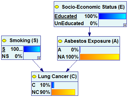
We can see that once the observation of smoking and education have been made, the marginal probability of Lung Cancer changes from 2% (a-priori probability) to 10% (a-posteriori probability).

Complex models allow for asking questions similar to the ones asked of the simple example network. And so, in case of the Diesel locomotives example, we can ask the probability of any fault given a set of symptoms or test results, we can ask for the most probable faults, and the most effective questions to be posed in order to reach a final diagnosis.

The following network (Hepar II) models common diseases of the liver: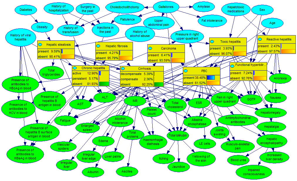

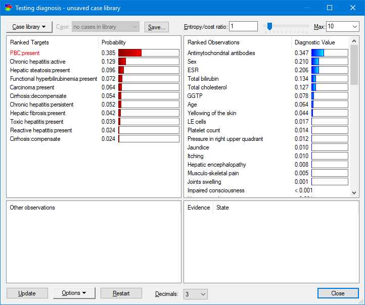
Special diagnostic dialog allows for viewing the diseases (upper-left pane) from the most to least likely and the possible observations and medical tests rank-ordered from the most to least informative given the current patient case.

This is all straightforward to compute from the joint probability distribution represented by the Bayesian network.

Embedding Bayesian networks technology into your software

Bayesian networks can be embedded into custom programs and web interfaces, helping with calculating the relevance of observations and making decisions. SMILE Engine, our software library embedding Bayesian networks, has been deployed in a variety of environments, including custom programs, web servers, and on-board computers.