What are Influence Diagrams?

Influence diagrams (IDs) introduced by Howard and Matheson (1984), are acyclic directed graphs modeling decision problems under uncertainty. An ID encodes three basic elements of a decision: (1) available decision options, (2) factors that are relevant to the decision, including how they interact among each other and how the decisions will impact them, and finally, (3) the decision maker’s preferences over the possible outcomes of the decision making process. These three elements are encoded in IDs by means of three types of nodes: decision nodes, typically represented as rectangles, random variables, typically represented as ovals, and value nodes, typically represented as diamonds or hexagons. Most popular type of IDs are those in which both the decision options and the random variables are discrete. A decision node in a discrete ID is essentially a list of labels representing decision options. Each random variable is described by a conditional probability table (CPT) containing the probability distribution over its outcomes conditional on its parents. Each value node encodes a utility function that represents a numerical measure of preference over the outcomes of its immediate predecessors. IDs can be viewed as an extension of Bayesian networks with an explicit representation of decision options and preferences over the possible outcomes of the decision process.

If you want to see live influence diagrams in action, visit our online model repository at https://repo.bayesfusion.com and select “Influence diagrams” category from the drop-down list located in the top-left corner of the window.

The structure of an influence diagram and its interpretation

It is convenient to view influence diagrams as extensions of Bayesian networks. While Bayesian networks are models of real-world systems in terms of representing the ties among the model variables (roughly speaking, this is what the joint probability distribution is about), the additional elements serve to represent explicitly both decision options and consequences of the decisions. Consider the following model, which is a simple extension of the example described in the Bayesian networks section.

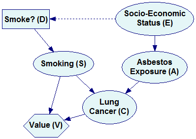
In addition to the variables E, S, A and C, modeling the interaction among smoking, asbestos exposure and lung cancer, the model includes two new nodes: (1) A decision node Smoke? (D), representing a decision option whether or not to smoke, and (2) a utility node Value (V) that is a function of nodes C and S and expresses the decision maker’s valuation of various outcomes of the decision process. Node D impacts directly only the variable S. S, in turn, impacts indirectly both C and the value (V) of the decision making process. The value is influenced by both S (the pleasure derived from smoking) and C (developing lung cancer). The dashed arrow from the variable E to D is called an information arrow and represents the fact that the decision maker knows the state of E before making the decision D. Knowing the states of some of the nodes in the model can impact the decision.

​The definition of D is rather simple. Because it is a discrete node, it’s domain is a set of two possible states, Smoke and DontSmoke.

Because the node S has a new parent, D, its definition changes from the original specification of the prior probability distribution to the following:

This new definition essentially states that once the decision maker has decided whether to smoke, she will follow up on this decision with certainty. Should we want to model possible difficulties with implementing the chosen decision, the table could contain parameters between 0 and 1. An alternative approach would be to convert the node S into a decision node.

​The definition of the node V is a deterministic function of the variables S and C. Essentially, the decision maker’s valuation of the outcomes of the decision making process depends only on these two variables. Smoking is preferred over not smoking because of the additional pleasure drawn from it. Having no lung cancer is preferred over the having cancer. Valuation of the outcome of the decision is a function of these two. Consider the following definition of V:

While the numerical valuation of the outcomes can be expressed in easily measurable units, such as money, in our model they are numbers on a scale between 0 and 100, expressing relative valuation of the outcomes. There is a well developed theory, dating back to early 20th century, for measuring the value of outcomes of a decision process known as the Expected Utility Theory. Roughly speaking, valuation of outcomes of a decision process is always relative to the decision context and is determined up to a linear transformation, which implies that it has neither a unit nor a zero point. It is customary to express utility on a scale from 0 to 100, where 0 is is the value of the worst possible outcome and 100 is the value of the best possible outcome. In our decision problem, the worst possible outcome is when the decision maker decides not to smoke but still develops lung cancer. The best possible outcome is when the decision make decides to smoke, draws enjoyment from smoking, and yet does not develop lung cancer. Smoking and developing lung cancer and not smoking and not developing lung cancer are placed on this scale at 5 and 95 respectively. Once the worst and the best possible outcomes have been identified and assigned the values of 0 and 100, numerical values for the remaining outcomes can be obtained through a well developed and studies process of utility elicitation.

Reasoning with influence diagrams

A decision model, as specified above, can be evaluated. Evaluation amounts to calculating the expected utilities for every combination of decisions. In the above example, we have only one decision with two states, so evaluation will amount to calculating the expected utilities of each of the two states. In GeNIe, these expected utilities can be viewed in the Value tab of the decision node D:

or the Value tab of the value node V:

In both cases, the results are conditioned on the value of the node Socio-Economic Status (E). The state of the node E is knows when the decision is being made, as expressed by the dashed arrow in the graph and explained earlier. In general, the decision whether to smoke or not may be different for the two population groups. In each case, i.e., for every possible state of the node E, the decision option that results in the highest expected utility (shown in bold font) is the one that is optimal and that should be advised. In our example, whether the decision maker is educated or uneducated, she should not smoke, as the expected utility of not smoking is higher than the expected utility of smoking.

Causality and influence diagrams

Similarly to Bayesian networks, directed graphs of influence diagrams are capable of expressing causality. While the pure mathematical formalism of Bayesian networks does not require arcs to be causal, in influence diagrams all arc originating in decision nodes are causal and express the fact that making a decision impacts the nodes at the other end of the arcs. When the arc is pointing to a chance node, that chance node is going to be impacted by the decision. When the arc points to a value node, it means that the decision impacts the value directly.

Embedding influence diagrams technology into user programs

Similarly to Bayesian networks, influence diagrams can be embedded into custom programs and web interfaces, helping with calculating the relevance of observations and making decisions. SMILE Engine, our software library embedding Bayesian networks, has been deployed in a variety of environments, including custom programs, web servers, and on-board computers.